Introduction to Pairs Trading
The primary goal in an investment endeavor is the implementation of strategies that minimize the risk while also maximizing the financial gain or return from the said investment. While there have been many popular strategies and techniques developed over the years that point towards the same goal, the 'Pairs-Trading' strategy is one that has been used to great extent in modern hedge-funds, for its simplicity and inherent market-neutral qualities. This strategy, often termed a statistical-arbitrage, relies on monitoring the correlation between a pair of stocks (known to be correlated). A long position is opened on the stock that rises and a short position is opened on the stock that falls. The underlying assumption in pairs-trading is that pairs of stocks, that have historically shown similarities in their behavior will eventually converge in the long run, even if they diverge in the short term, allowing the trader to profit off the pair regardless of the market.
In such a strategy, identification of correlated stocks and generation of pairs is of paramount importance. In this project, we employ unsupervised learning techniques that include Density-Based Spatial Cluster of Applications with Noise and K-Means Algorithm. Once, the relevant pairs have been identified, their price relations are extrapolated using supervised learning techniques such as Linear Regression. This overall methodology will help provide insight into the relations between various stocks and facilitate the generation of appropriate trading strategies for them.
Dataset
The datasets are provided by Wharton Research Data Services (WRDS). We mainly obtained the daily stock files from file from CRSP and quarterly fundamentals from Compustats for our purpose. Initially, our dataset consists of stock price files from 3000 stocks which are constituents of Russell 3000. Those stocks' value and size are large enough to restore the whole market value, representing approximately 95% of the total market shares. We performed this pre-screening process to avoid the 'small-cap' trap in the market. Currently, there are more than 6000 active stocks in the U.S. Stock Market but most of them are micro-valued. In reality, investors often cautiously avoid investing in those stocks, since trading, even a small number of shares might have unpredictable effects on their stock prices. We should keep this in mind when doing academic research. We set the sample period from 2010-01-01 to 2015-12-31 for training strategies and use sample period 2016-01-01 to 2019-12-31 for backtesting.
Data Processing
Data Preprocessing
In our next stage, we want to pre-select eligible stocks that enable us to sail through further steps. First, we removed stocks that were delisted, exchanged, or merged during our sample period since those stocks are no longer tradable. Next, we removed stocks that have negative prices which will be problematic for further analysis. Stocks that are constantly trading at-low-volume also have to be removed since improper trading executions can largely change their stock prices and altered history. Finally, we remove stocks that have more than half missing prices, so that we have enough available data for imputation. A similar approach was performed on the financial fundamentals of datasets. In the end, there are 1795 eligible stocks for further analysis.
Data Imputation
In this step, we imputed the missing values in our preprocessed dataset. We worked with the time series data and the financial ratios separately. We imputed both of them using means, although in a slightly different way. For the time series data of stock prices, missing values were replaced by the mean of all the available stock prices for that stock in the training period. Since the financial ratios individually have different bounds we imputed missing values in the financial ratios dataset with the average of all available data for the particular ratio.
Dimensionality Reduction using Principal Component Analysis
Considering that we have more than 2000 features in the imputed dataset (which inlcudes both realtime stock data as well as several financial ratios), it is pertienent for us to use dimensionality reduction so that we can feasibly run unsupervised learning algorithms in the subsequent steps. It should also be noted that each datapoint in the time searies data is considered to be 1 individal feature. We used Principal Component Analysis (PCA) to reduce the dimensionality while retaining majority of the variance from the dataset. Once again, we performed PCA independantly on the time series stock price data and the financial ratios. After PCA, the time series data is reduced to 15 principal components and the financial ratios are reduced to 5 principal components. We retained more than 99% of the variance in either case. Here are two plots illustrating the proportion of variance captured by the top singular values:
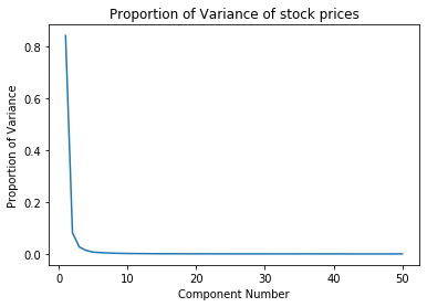
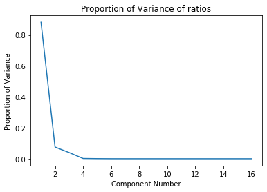
We made sure to choose the number of principal components coming from the price dataset to theone coming from the financial ratios becausewe primarily want to rely on the stockprices in order to perform the clustering. The resultant reduced datasets are then concatenated to create a 20 dimensional training dataset which we then use for clustering analysis.
Two clustering algorithms were explored to create clusters of stocks:
KMeans Clustering
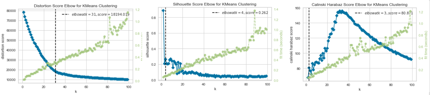
The KMeans clustering algorithm is a popular clustering methodolgy. The most important aspect of this algorithm is the determination of the number of clusters. This can be ascertained using an elbow-method based cross-validation technique. There are three loss-metrics (or scores) that can be used in the elbow method which are:
- Distortion Score: computes the sum of squared distances from each point to its assigned center (smaller is better)
- Silhouette Score: calculates the mean Silhouette Coefficient of all samples (smaller is better)
- Calinski Harabz Score: computes the ratio of dispersion between clusters to dispersion within clusters (larger is better)
The dataset is first normalized before the elbow analysis is carried out for each of the scores mentioned above, the results of which are shown below. The elbow for each of the analyses are also indicated. It should be noted that the elbow is determined using a built-in “knee point detection algorithm”. This algorithm sometimes converges on a local minima/maxima giving erroneous elbows, as is evident from the Calinski Harabz Score where the global maxima is approximately 30. The maximum cluster number from each of these independant metrics was finally used in training the KMeans Algorithm. In this case, the max cluster elbow among the three was 31 which is what was finally chosen as the number of clusters in the training. Choosing a max among the three is based on the intention of making each cluster as small and isolated as possible.
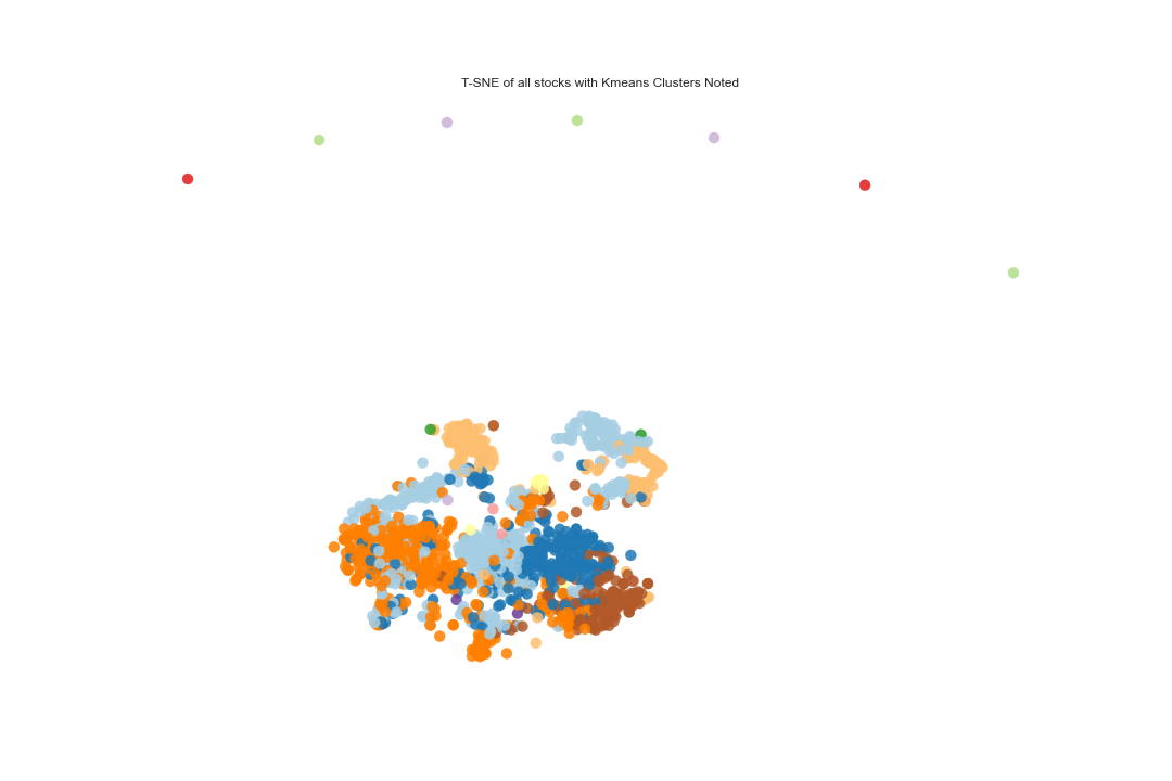
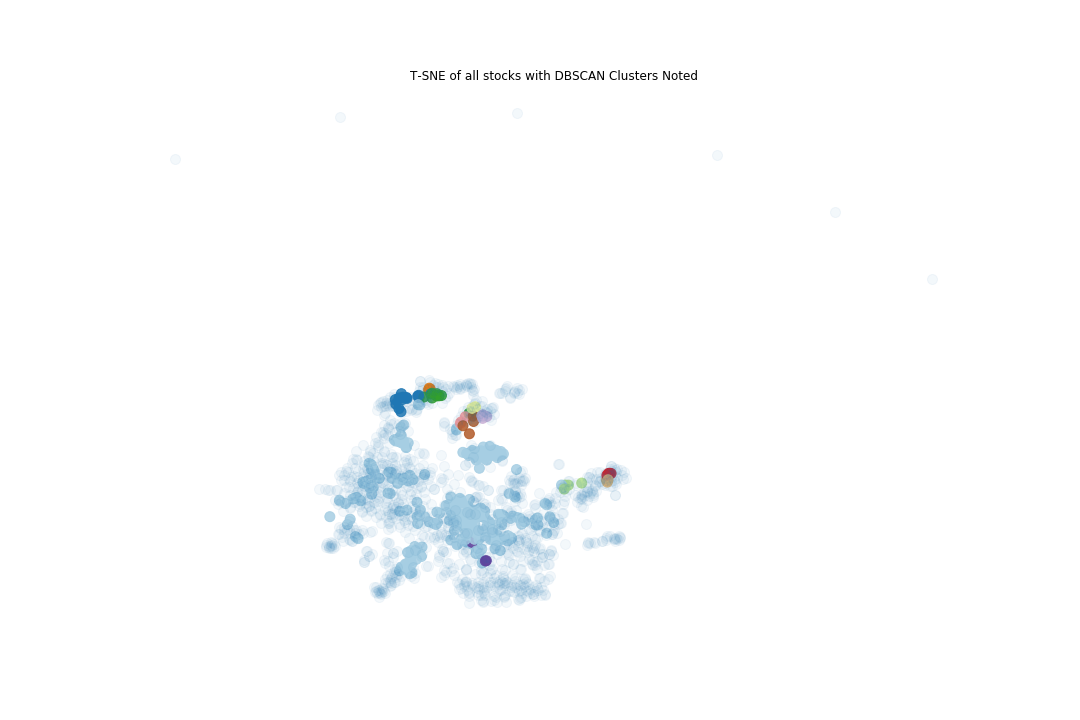
The following plot shows a visualization of the clustered datapoints in the form of a t-Distributed Stochastic Neighbor Embedding (t-SNE) plot. t-SNE is a non-linear dimensionality reduction algorithm used for mapping multi-dimensional data to two or more dimensions that makes it easier to visualize the clusters. The number of stocks in each cluster is also illustrated below. We notice a slight disproportionality in the size of each cluster. This disproportionate distribution of the stocks in clusters is expected, to some extent, since the dataset is possibly dominated by stocks from a single or closely related industries.
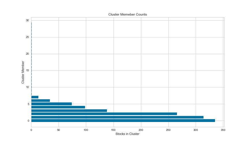
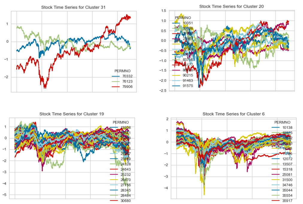
In order to increase confidence in the clustering procedure, the real time series stock price data of the stocks in each cluster were also investigated. The time series data of the stocks in 4 of the 31 clusters are illustrated below. Since some clusters have too many stocks in them to properly visualize, the number of stocks in each time series plot is restricted to 100 for convenience. The From a visual perspective, stocks within the same cluster do show a good correlation among them in terms of the behavior of the stock prices.
Density-based spatial clustering of applications with Noise (DBSCAN)
The DBSCAN algorithm was paramterized by eps = 1.8 and minPoints = 3 which resulted in the formation of 11 clusters. A simple visualization of the cluster in the form of a T-SNE plot is shown below:
The following figure shows the number of members in each cluster, demontrating the fact that a huge proportion of the stocks are bunched into a single cluster.
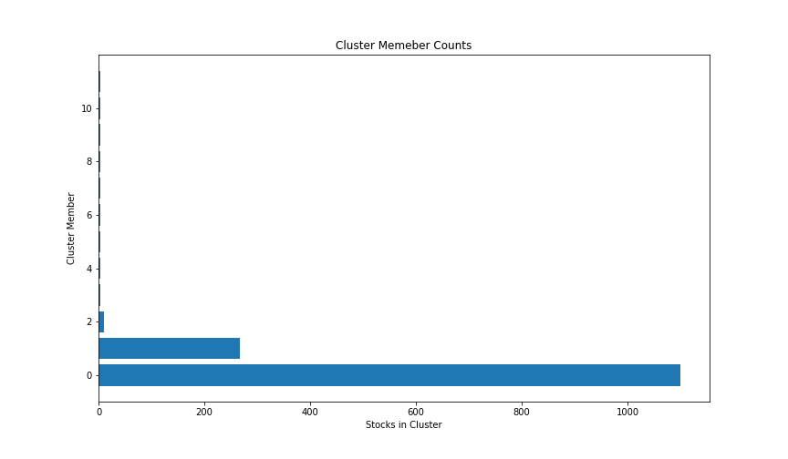
Once more, we plot a few of the time series data points of stocks within the same cluster for confidence. From a visual perspective, stocks within the same cluster do show a realtively high correlation among them in terms of the behavior of the stock prices.
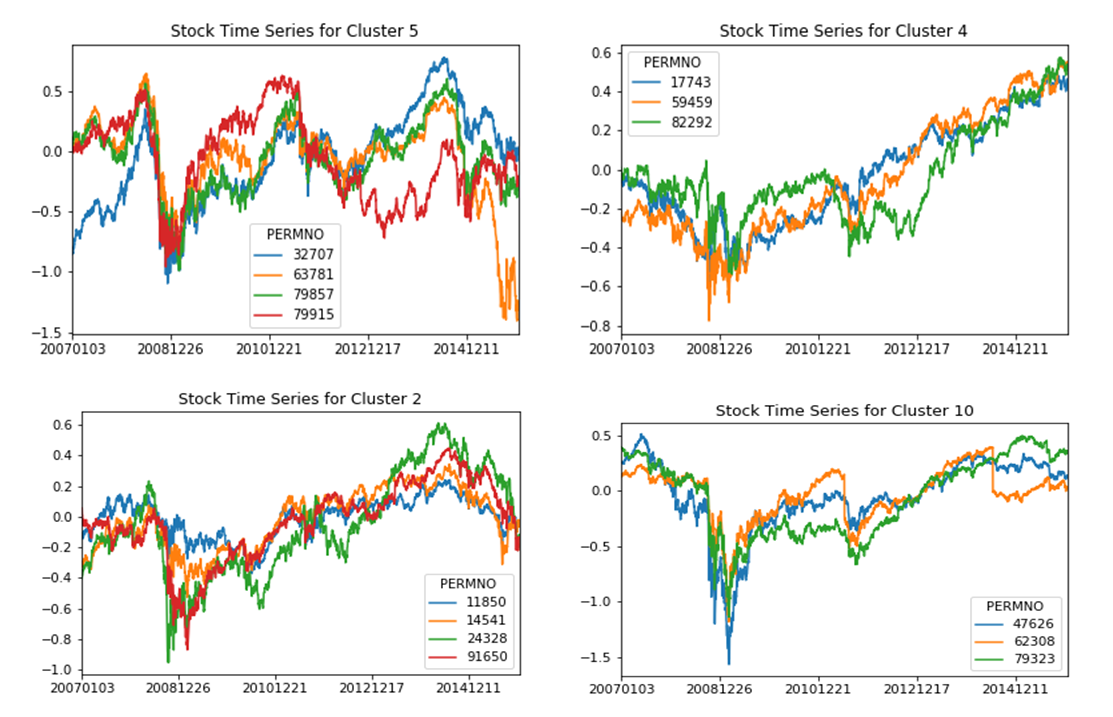
Due to time constraints, only the clustering from the DBSCAN algorithm was finally used to generate optimized pairs that were analysed in the subsequent strategy implementataions
Pair selection
The key of finding valid pairs is to find the cointegration of two selecting stocks. As we will go in detail later, we want to find two stocks that their time series of prices follows a linear relationship but not always. The spread of two selecting stocks should be a mean-reverting process, meaning that their spread tends to drift towards its mean function over time. The Ornstein–Uhlenbeck process is a mean-reverting process that commonly used in the field of financial mathematics. Here in our project, we also take the idea of O-U process to compute the spread and model the relation of stocks.
To find such pairs, we performed ADF test (or Augmented Dicky Fuller Test) to every pairs in each clusters to find cointegrated pairs. ADF test is usually used in time series analysis. In this case, ADF test helps us determine whether the spread of two stocks is stationary or not. A stationary process is very valuable to model Pairs Trading strategies. For instance, in this case, if the spread is stationary, we know that the difference in their stock process will drift to the mean (which is zero in our case) over time if it is temporarily derailed, and this is the time window for us to make money.
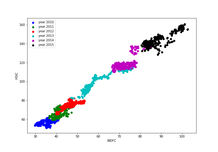
Take WDFC and HSIC as an example. The relationship of their stock price over time is illustrated below.
We performed ADF test to their spread as we defined in next section and plot the time series process of their spread.
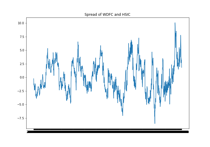
The ADF test gives p-value as the result. For this pair, the p-value is 2.8702051939237176e-05, which is less than significant level 0.05 (as we set). Thus, we are over 95% confident to say that the spread of WDFC and HSIC's stock price is stationary and they are valid pair.
We performed such test to all pairs and select at least one pair in each cluster to diversity our portfolio. Then, a strategy that observed based on the movement of the spread can be designed and executed well in the later part.
Trading Strategy
In this section, we will discuss how we generate the z-score history by stock pair's price history. We generate the z-score history to decide when we long and short the stocks. The z-score is simply (spread)/(standard deviation of spread) and spread is calculated based on the stock pair's price history. The basic method to calculate the spread is using a log of prices of stocks A and B. Spread = log(a) - nlog(b), where 'a' and 'b' are prices of stocks A and B respectively. The 'n' is the hedge ratio which is constant. We used the machine learning to calculate the spread instead of the log. It will be discussed in the following sections.
Linear Regression
We used the log of stock A's prices as data points and the log of stock B's prices as a label. We train the polynomial regression model with these datasets.
Regularization
For the regularization of the model, we used the LASSO regression. We used the LASSO regression instead of Ridge regression because not only punishing high values of the coefficient but actually setting them to zero if they are not relevant. (Ridge vs Lasso)
Validation
In the model, we have two hyperparameters. First one is alpha in the Lasso regression and the other one is a degree of the polynomial regression. The scikit-learn library already has a module about cross-validation for the alpha in the Lasso function. It uses the K-fold method. In a case of degree, we did the validation by ourself. First we pick the 66% of datasets as training data. This pick was random because the relation of stock a and b can be changed by time. Then, we used the 33% of datasets as validation data and calculate the RMSE. By comparing the RMSE, we choose the degree.
Function
After we generate the model, we predict the log(b) and calculate the spread as:
Spread = lr.pred(log(a)) - log(b)
It also leads us to calculate the z-score by the following equation:
z-score = Spread / standard deviation
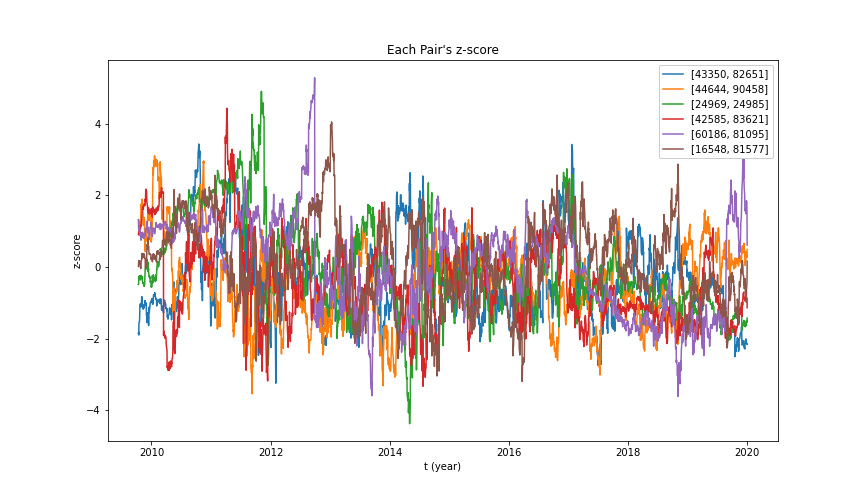
The standard deviation is calculated by training data, which is the training data prices' spread history. We also used the degree = 4 for the polynomial linear regression hyperparameter. If it becomes too big, it goes to overfitting and will not generate the spread. If the spread distribution is small, it is hard to decide when we long and short the stocks. Here is the example graph of z-score history for the stock pairs we have. You can see it converges.
Backtesting
In this section, we will discuss testing. We apply our trading strategy to the real stock market and check how much we can earn based on our approach. We used the moving windows approach for the testing. For the training data, we used the previous 700 days stock prices. After we train the model with our machine learning algorithm, we calculate the z-score with the generated model and decide whether we will long or short the stocks. The input of backtesting is the z-score history generated in the 'trading strategy' part and the price history. Based on the input, we keep calculating the earning and loss of our stock and inverse. We also track the total asset history and return it as an output of backtesting.
Implementation
To simplify the backtesting, we just set the initial money as million dollars and the volume of the stocks we trading as 'total assets' / '# of pairs'. Therefore, if our current total asset is $100 and the number of stock pairs is 10, we long/short the stock only with $10. We also calculate the price of the inverse (short) in the everyday base and we didn't consider the commission of trading to simplify.
Results
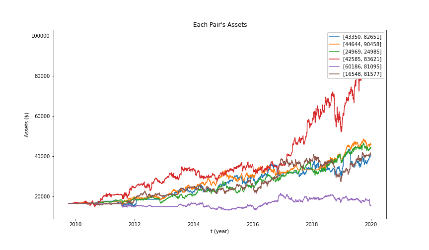
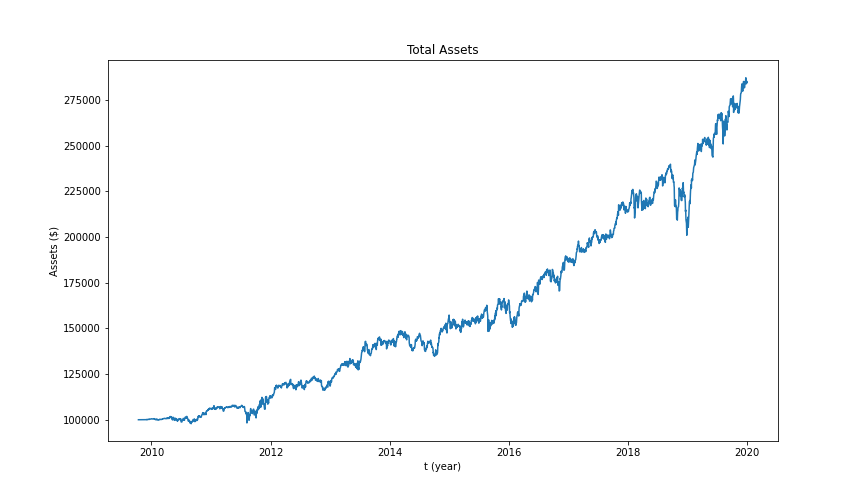
We run the backtesting for all the timeline (2007~2015). Here are all the results from the backtesting. The x-label is the daily based time. It does not include market off-day. The y-label is the money (dollars).
Each pair's assets linear regression
Total assets linear regression
Linear Regression with Kalman Filter
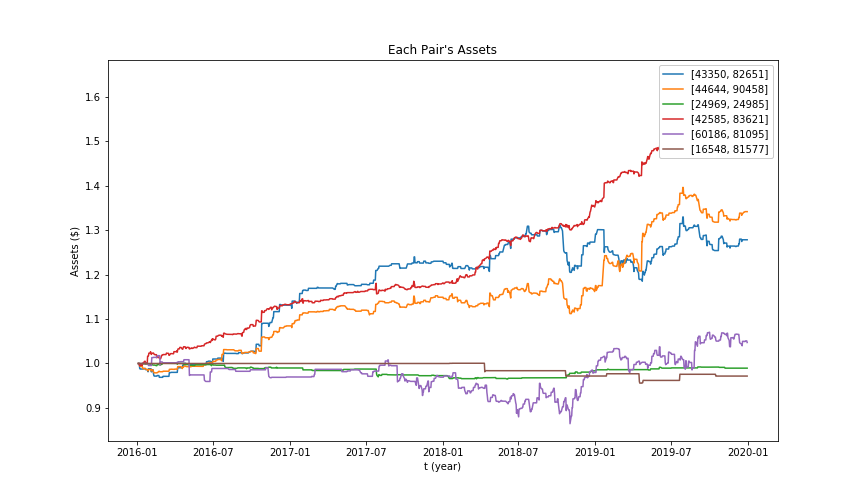
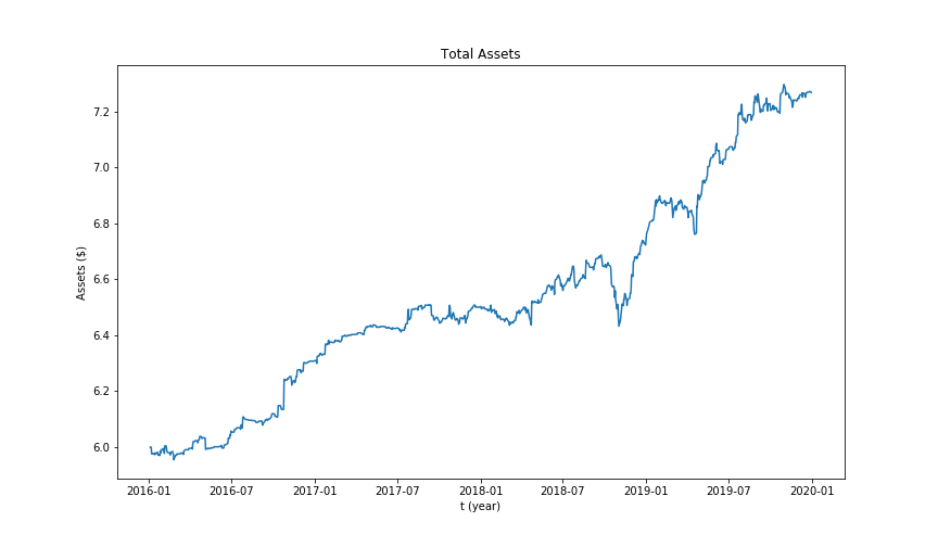
We also used Kalman filter as an online linear regression method. (We used qstrader platform for backtesting and implementation)The idea is to assume linear relationship between the prices of the related assets. We keep updating the relationship at each step on testing data based on the previous results instead of traditional machine learning approach. At each step we take actions upon excessive deviation from the predicted price and the real price. The idea is to assume future convergence of the related stocks' prices. Included below are results of some of the pairs. Not all of them are satisfying and, rather, some even would suffer significant losses over the testing period. The portfolio as whole, however, has decent performance. We searched through possible action threshold pairs to find the optimal performance upon testing.
Each pair's assets kalman filter
Total assets kalman filter
Performance Evaluation and Conclusion
The following table gives some performance metrics of strategies with Linear Regression and Online Linear Regression (Kalman Filter). Note that those metrics are evaluated only through testing period, which is from 2016-01-04 to 2019-12-31, to be more represensitive.
| Metric | Linear Regression | Kalman Filter |
|---|---|---|
| Maximum Drawdown | -16.2044% | -3.6690% |
| Alpha | 20.0352% | 6.3747% |
| Beta | -0.2437 | 0.2065 |
| Annual Volatility | 0.1241 | 0.02758 |
| Sharpe Ratio | 1.1969 | 3.1478 |
| Sortino Ratio | 1.7190 | 5.2359 |
The above statistics show that Linear Regression has better alpha performance (excess return) than Kalman Filter, which is 20% versus 6.374%. However, Kalman Filter undertakes lower risk while it still maintains relatively satisfying performance. Preference of strategies highly depends on investor's level of risk aversion. A risk taker can bare up to -16% loss of investment and he/she might prefer Linear Regression. A risk averse person, on the other hand, might favour Kalman Filter for its lower risk undertaking. However, for the moment, Pairs Trading Strategy has demonstrated its high investment potential especially with the advanced statistical analysis. Researchers can further investigate in this field to achieve better alpha performance and lower risk at the same time.
Contribution
- Daehyun Kim
- Trading Strategy Structure
- Trading Strategy Algorithm (Linear Regression)
- Backtesting
- Xin Yi
- Data Collection and Preprocessing
- DBSCAN Algorithms for Clustering
- Cointegration test and Pair Selection
- Performance Metrics
- Nael Mizanur Rahman
- KMeans Clustering Algorithms, Cluster Evaluation and Cluster visualization
- Sudipta Kolay
- Data Imputation
- Dimensionality Reduction using Principal Component Analysis
- Zhenyu Jia
- Kalman filter strategy implementation and backtesting
All members constibuted to the final project report.
Reference
https://blog.quantinsti.com/pairs-trading-basics/
https://en.wikipedia.org/wiki/Pairs_trade
https://www.quantstart.com/articles/kalman-filter-based-pairs-trading-strategy-in-qstrader/
https://hackernoon.com/practical-machine-learning-ridge-regression-vs-lasso-a00326371ece